In geophysics, we often work with instrument responses in the frequency domain as they are simpler to combine and manipulate For instrument responses specified in the time domain, we must first transform the response of the frequency domain using one or more transforms. Depending on the application, one or more of the following transforms may be used: The Fourier Transform, the Laplace Transform and the z-Transform.
The Fourier Transform
Introduction
The Fourier Transform (\(t \rightarrow \omega\)) is defined by
while the Inverse Fourier Transform (\(\omega \rightarrow t\)) is given by
There are different conventions in use for the Fourier Transform. The conventions differ in which transform (forward vs. reverse) has the positive sign in the exponent, and which transform is scaled by \(\frac{1}{2\pi}\). Some authors prefer to scale each transform by \(\frac{1}{\sqrt{2\pi}}\) instead. What is important is that forward and reverse transforms must have exponents that are opposite in sign, and the product of the scale factors must equal \(\frac{1}{2\pi}\).
Discrete Time Fourier Transform (DTFT)
In the Fourier transform pair above, both time (\(t\)) and frequency (\(\omega\)) are continuous parameters. In contrast, for signals sampled discretely in time, we may define the related Discrete Time Fourier Transform (DTFT) as
where \(n\) is the discrete sample number, and \(\omega\) is still continuous.
Discrete Fourier Transform (DFT)
And finally, when both time and frequency are discrete, we define the Discrete Fourier Transform (DFT) pair by
Note that the popular Fast Fourier Transform (FFT) is a particular implementation of the DFT.
The Laplace Transform
Introduction
The Laplace Transform is defined by
If we make the substitution, \(s=\sigma + j\omega\), this becomes
Each point in the complex s-plane is associated with a frequency, \(\omega\) and an exponent \(\sigma\). Thus, each point in the s-plane describes a sinusoid of frequency \(\omega\) that is either exponentially growing (\(\sigma>0\)) or exponentially decaying (\(\sigma<0\)) with time.
Note that the Laplace transform evaluated along the imaginary axis (where the attenuation parameter, \(\sigma=0\)), reduces to the complex Fourier transform, \(X(\omega)\).
The Laplace transform at point \(s\) is a measure of the similarity between the input signal, \(x(t)\), and the corresponding exponentially growing/decaying sinusoid. A large value of \(X(s)\) corresponds to a strong similarity between the input signal and the sinusoid \(e^{-(\sigma + j\omega)t}\), indicating a strong presence of the sinusoid in the input signal.
In practice, we are often only interested in causal signals that begin at \(t=0\). Using the unit step function,
we may ensure causality by writing \(x(t)=u(t)x(t)\) , so that the Laplace Transform becomes
Poles and Zeros
Suppose we have a data processing system (e.g., analog sensor + datalogger) that can be characterized by the linear differential equation,
where \(x(t)\) is the input signal (e.g., the ground motion), \(y(t)\) is the output signal (the signal recorded) and \(a_{k}\) and \(b_{k}\) are constant (time-invariant) coefficients. If we assume the system is causal, so that the signals + derivatives are all 0 for \(t<0\) , then the Laplace Transform of the equation gives
or
From this we can write the system transfer function relating the output to the input as
or more generally,
This is the coefficient representation of the transfer function. It represents the transfer function as the ratio of two polynomials. The roots of the numerator polynomial are called ‘zeros’, while the roots of the denominator polynomial are called ‘poles’.
Often, for analog stages, it is more convenient to factor the transfer function in terms of these poles and zeros:
where \(z_{k}\) are the M zeros of the system, and \(p_{k}\) are the N poles.
Because the coefficients of the numerator and denominator polynomials are real, the corresponding roots (poles and zeros) must occur in complex conjugate pairs.
Thus, the poles and zeros are either real or form pairs that are symmetric with respect to the real axis in the complex \(s\)-plane. In addition, it can be shown that for systems that are stable and causal, the poles all have real parts \(\le 0\).
Recall that the Laplace transform variable is given by \(s=\sigma+j\omega\). Along the imaginary axis, \(\sigma=0\) and hence \(s=j\omega\). Thus, we may express the complex frequency response of the analog stage by calculating its polezero expansion
where \(s=j2\pi f\) [rad/s] or \(s=jf\) [Hz].
Thus, given the poles and zeros of an analog stage, in order to properly calculate the stage frequency response, we must know the units of \(s\) used to calculate the poles and zeros.
In StationXML, these units are specified by the PzTransferFunctionType element within the PolesZerosType response stage:
<Stage number="1">
<PolesZeros>
   ...
   </OutputUnits>
      <PzTransferFunctionType>LAPLACE (RADIANS/SECOND)</PzTransferFunctionType>
      <NormalizationFactor>1.0</NormalizationFactor>
      <NormalizationFrequency unit="HERTZ">1.0</NormalizationFrequency>
where the possible values for PzTransferfunctionType are:
“LAPLACE (RADIANS/SECOND)”
“LAPLACE (HERTZ)”
“DIGITAL (Z-TRANSFORM)” (Discussed in next section)
Note also the <NormalizationFrequency> with unit “HERTZ”. These units are distinct from those used to identify \(s\) above. The <NormalizationFrequency> specifies the frequency (in Hz) at which the polezero transfer function is normalized. The recommended practice is to choose a value of normalization factor, \(A_0\), that normalizes the polezero expansion to unity at the specified normalization frequency, \(f_n\):
The z-Transform
Introduction
The z-Transform is defined by
where
Notice that on the unit circle, where \(|z|\equiv |r|=1\) and \(z=e^{j\omega}\) , the z-transform reduces to the discrete Fourier transform (DTFT):
The z-transform measures the similarity between the input signal \(x[n]\) and the signal \(z^{-n}\).
\(z^{-n}\) represents exponentially increasing (for r < 1) or decreasing (r > 1) sinusoids. e.g., \(e^{-j\omega n}\) is a sinusoid with angular frequency \(\omega\) [radians/sample] that expands with sample number n.
Thus, the location (value) of \(z\) in the complex plane controls what \(z^{-n}\) looks like.
The fractional or angular frequency, \(\omega\) [radians/sample] is related to the linear frequency of the sinusoid through
so the number of samples/cycle is given by
and this corresponds to a period of \(T=N\Delta t\) [seconds],
where \(\Delta t\) is the sampling interval (secs) and is related to the sampling rate by: \(f_{s}=\frac{1}{\Delta t}\). Then the frequency of oscillation is given by \(f=\frac{1}{T}=\frac{1}{N\Delta t}=\frac{f_{s}}{N}\) [Hz]
In other words, as the angle in the complex z-plane goes from \(\omega=0\) to \(\omega=\pi\), the linear frequency goes from \(f=0\) to \(f=f_{Nyq}\) [Hz], where the Nyquist frequency, \(f_{Nyq}=\frac{f_s}{2}\) [Hz].
Thus, in implementing the frequency response of the z-transform (e.g., when calculating the response of a FIR filter), it is common to write it in a way that removes the dependency on the actual sample rate, or
Difference Equations
z-transforms of linear time-invariant (LTI) systems described by difference equations play an important role in signal processing.
The general form of a difference equation is:.
where \(a_{0}\ne0\) (the coefficient of y[n] can’t be zero)
Taking the z-transform of both sides,
or
From this we can write the system transfer function
The transfer function is the z-transform of the system impulse response, \(h[n]\), or
The transfer function can also be factored in terms of poles and zeros (for \(b_{0}\ne0\))
where \(c_{k}\) are the M zeros of the system, and \(d_{k}\) are the N poles.
For a system to be both stable and causal, its poles must lie inside the unit circle, or \(|d_{k}|<1\) for \(k=1,N\).
z-Transform Frequency Response
How does the location of the poles and zeros of the z-transform influence the complex frequency response, \(H(f)\) ?
We start by only considering the magnitude response, \(|H(f)|\).
The z-transform only exists within a region of the complex z-plane where the infinite sum converges. We call this region the Radius of Convergence (ROC) of the system.
If our system, described by difference equations, is stable, then the ROC must include the unit circle, \(|z|=1\) where
The magnitude of the product is equal to the product of the magnitude, thus
In other words, as we traverse the unit circle through circular ‘frequency’, \(\omega\), from \(0-2\pi\), the magnitude of the response depends on the distance between the point on the unit circle, \(e^{j\omega}\), and the zeros, \(|e^{j\omega}-c_k|\), as well as the distance between the point and the poles, \(|e^{j\omega}-d_k|\), or
Thus, \(|H(e^{j\omega})|\) is small when \(e^{j\omega}\) is near the zeros and it is large when \(e^{j\omega}\) is near the poles.
Examples
Example 1
Consider a system with zeros at \(z=1,-1\) and poles at \(z=0.95e^{\pm j\pi/4}\), with response function
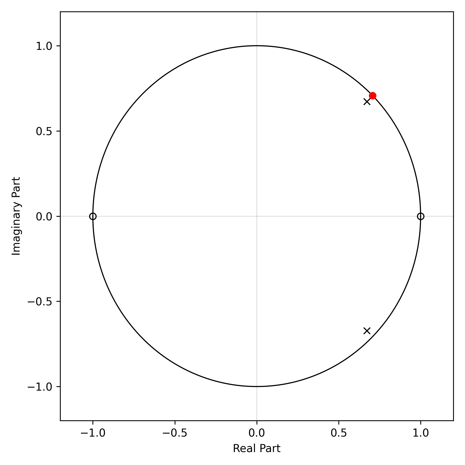
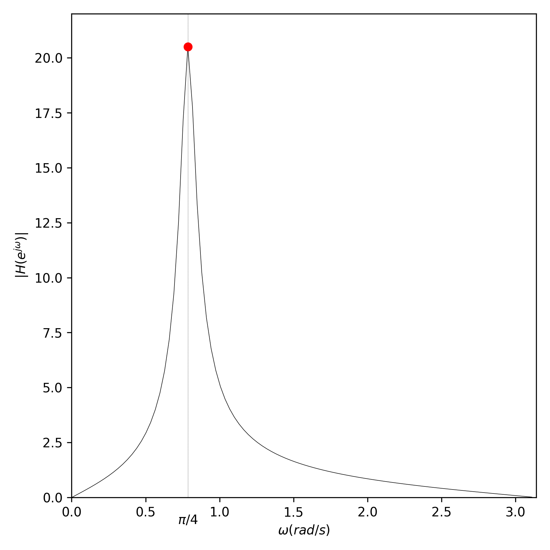
Poles near the unit circle push the magnitude response up at those frequencies, while zeros near the unit circle pull it down; if the zero is actually on the unit circle, then it forces the magnitude response to be exactly 0 at that frequency.
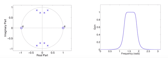
Example 2
Here’s an example pass-band filter comprised of 8 poles and 8 zeros. We can predict from the position of the poles and zeros that the frequency response will be 0 at \(\omega=0\) and will be maximum near \(\omega=\frac{\pi}{2}\).
FIR-IIR Filters
Introduction
As we’ll see in the next section, each of the multiple stages that comprise an instrument response can be thought of as a filter that modifies the amplitude and phase of the original signal (e.g., ground motion) in some way.
In fact, to truly understand instrument response and data processing in general, it is necessary to have some familiarity with digital signal processing.
There are two categories of discrete-time filters that we routinely encounter in seismology:
FIR filters (Finite Impulse Response)
IIR filters (Infinite Impulse Response)
Both filters can be constructed using difference equations, hence, they are often represented in terms of their z-transforms.
FIR filters can be written as:
while IIR filters can be written as:
FIR filters can be thought of as a sum of weighted values of past inputs, \(x[n-k]\) (the so called moving average filter). IIR filters have this same moving average component, but also offer the possibility of feedback, since the current output \(y[n]\) can also depend on a weighted combination of past outputs, \(y[n-k]\).
For a finite input impulse, the subsequent impulse response of a FIR filter is finite. However, because of the dependence on past outputs, the impulse response of the IIR filter is, at least in theory, infinite; it continues long after the input signal has finished.
In the FIR case, the system function, found by taking the z-transform of the difference equation, can be written
while for the IIR case, the system function is
where \(a_0=1\).
The system functions can be factored in terms of their poles and zeros as
Thus, the FIR filter has arbitrary zeros, but only has poles at the origin (\(z=0\)). However, poles (or zeros for that matter) at the origin don’t affect the frequency response since they are located a fixed distance (\(|z|=1\)) from the unit circle.
In contrast, the IIR filter may have both zeros and poles at arbitrary locations, making them especially flexible.
The corresponding impulse responses are found by taking the inverse z-transform of the system functions,
Thus the FIR impulse response is given by the difference equation coefficients, \(b_k\), themselves, and the impulse response dies after \(M\) terms.
The impulse response of the causal parts of the IIR filter can be written as
where \(u[n]\) is the unit step function (\(u[n]=1,n\ge 0\)).
Because of the geometric series \(d_k^{n}\), the IIR impulse response decays but never actually reaches zero.
FIR vs IIR
The primary distinguishing factor between FIR and IIR filters is this:
FIR filters are guaranteed to have a linear phase response, which is much easier to deal with, while IIR filters have non-linear phase response.
Some pros and cons of each filter type is summarized below.
FIR Filters:
- Pros
Can be designed using optimization techniques to match a desired magnitude/phase response
Allow for arbitrary magnitude/phase response
Allow for linear or zero phase response (no distortion)
Are always stable
- Cons
Can require a large number of coefficients (e.g., \(M\approx 100\)) to achieve desired accuracy, particularly for steep filters.
IIR Filters:
- Pros
Can be implemented very efficiently - fewer coefficients than FIR for comparable frequency selective filter accuracy (e.g., \(M\approx N\approx 8\))
Filtering is fast
- Cons
Generally can’t use optimization techniques to design
Better approach is to start from a well-known analog filter design and transform it to discrete-time filter.
Limited to frequency selective filters (e.g., bandpass, high-pass, etc)
Phase is nonlinear (will always cause phase distortion within the passband)
Zero phase filters are impossible to implement exactly (you can get this by filtering forward + backward, but this can’t be implemented in real-time!)
In spite of the cons listed above, there are some instances where IIR filters are preferred. For instance, for implementing maximally flat selective filters (e.g., Butterworth bandpass filters) or for modeling the behavior of systems with feedback.
Nevertheless, the vast majority of filters encountered in seismic metadata are anti-alias filters used at each decimation stage of the digitizer, and the digital anti-alias filters most commonly used are linear phase FIR filters that produce a constant time shift.
Hence, in what follows we will concentrate on FIR filters.
Classification of FIR Filters
FIR filter frequency response can be written
where in the last expression, we identify the filter coefficients \(b_{k}\) as the impulse response values: \(h[k]=b_k\) to show that the output of the FIR filter is the convolution of the input signal \(x[n]\) with the filter impulse response.
It can be shown that the FIR filter response has generalized linear phase of the form,
where \(A(e^{j\omega})\) describes the real amplitude, \(\beta\) is a constant phase factor, and \(\alpha\) is the constant group delay.
A consequence of this constant group delay (also called phase delay) is that the shape of the input waveform is not changed; all frequencies are delayed the right amount so that they add together in the same way to form the output signal. The resulting output signal has the same shape as the input signal but is delayed in time.
- Some general observations about FIR filters are:
FIR filters contain as many poles as they have zeros.
The number of zeros (poles), \(M\), is called the order of the FIR filter
All the poles are located at the origin (inside the unit circle), hence FIR filters are said to be stable.
These poles don’t affect the magnitude of the frequency response, only the phase.
Note that a filter of order M has length M+1.
FIR filters with generalized linear phase are often divided into 4 types depending on whether the order M is even or odd, so that the number of points is either odd or even, and whether the impulse response (=FIR coefficients) exhibits even or odd symmetry about the middle point.
FIR filters with symmetrical impulse response are often called two-sided or acausal. As a consequence of the symmetry of the filter impulse response, the onsets of very impulsive signals (with energy at frequencies near the Nyquist cut-off for the FIR filter), may be contaminated by precursory (=acausal) oscillations.
Type I: M even
M even + even symmetry about the midpoint M/2
Note that in this case, there will be M+1 (odd) points in the filter and M/2 will fall on an index right in the middle:
\[h[k]=h[M-k],0\le k\le M\]We can write out the frequency response and use symmetry to simplify,
\begin{eqnarray} H(e^{j\omega})&=&\sum_{k=0}^{M}h[k]e^{-j\omega k} \\ &=&h[0]+h[1]e^{-j\omega\cdot1}+h[2]e^{-j\omega\cdot2}+...+h[M-1]e^{-j\omega\cdot(M-1)}+h[M]e^{-j\omega\cdot M} \\ &=&e^{-j\omega\frac{M}{2}}\Big[h[0]e^{+j\omega\frac{M}{2}}+h[1]e^{-j\omega\cdot1}e^{+j\omega\frac{M}{2}}+...+h[M-1]e^{-j\omega\cdot(\frac{M}{2}-1)}+h[M]e^{-j\omega\frac{M}{2}}\Big] \\ &=&e^{-j\omega\frac{M}{2}}\Big[h[0]e^{+j\omega\frac{M}{2}}+h[M]e^{-j\omega\frac{M}{2}}+h[1]e^{-j\omega\cdot1}e^{+j\omega\frac{M}{2}}+...+h[M/2+1]e^{-j\omega\cdot1}+h[M/2]\Big] \\ &=&e^{-j\omega\frac{M}{2}}\Big[h[0](e^{+j\omega\frac{M}{2}}+e^{-j\omega\frac{M}{2}})+h[1](e^{+j\omega(\frac{M}{2}-1)}+e^{-j\omega(\frac{M}{2}-1)})+...+h[M/2-1](e^{+j\omega}+e^{-j\omega})+h[M/2]\Big] \\ &=&e^{-j\omega\frac{M}{2}}\Big[h[0]2cos(\frac{M}{2}\omega)+h[1]2cos((\frac{M}{2}-1)\omega)+...+h[M/2-1]2cos(\omega)+h[M/2]\Big] \\ H(e^{j\omega})&=&e^{-j\omega\frac{M}{2}}\sum_{k=0}^{M/2}a[k]cos(\omega k) \end{eqnarray}where \(a[0]=h[M/2],a[1]=2h[M/2-1],...,a[M/2]=2h[0]\).
In general, \(a[0]=h[\frac{M}{2}]\), and \(a[k]=2h[\frac{M}{2}-k],k=1,...,\frac{M}{2}\).
The \(a[k]\) coefficients are real, hence the sum is real, and the response satisfies the generalized linear phase property:
\[H(e^{j\omega})=A(e^{j\omega})e^{-j(\omega\alpha+\beta)}\]Hence for Type I, the amp is: \(A(e^{j\omega})=\sum_{k=0}^{M/2}a[k]cos(\omega k)\), while the phase term is: \(e^{-j\omega\frac{M}{2}}\) and the corresponding group delay is: \(\alpha=\frac{M}{2}\).
Type II: M odd
M odd + even symmetry about the midpoint M/2
Note that in this case, there will be M+1 (even) points in the filter, hence the symmetry mid-point falls between two sample points.
\[h[k]=h[M-k],0\le k\le M\]By similar algebra as above, we can write the frequency response as
\[H(e^{j\omega})=e^{-j\omega\frac{M}{2}}\sum_{k=1}^{\frac{(M+1)}{2}}b[k]cos(\omega(k-\frac{1}{2}))\]where \(b[k]=2h[(\frac{(M+1)}{2}-k],k=1,...,\frac{(M+1)}{2}\).
Thus, this system also has group delay \(\alpha=\frac{M}{2}\).
Type III/IV anti-symmetric
Type III (M even) and Type IV (M odd) FIR filters exhibit anti-symmetry about the midpoint: \(h[k]=-h[M-k]\).
As a result, their expansions reduce to summation of sine functions and can’t be used to implement low-pass filters, hence they are not used for anti-alias filtering.
Practical Concerns
Thus, we normally use FIR filters of type I or II for anti-alias filtering. Because of their symmetry, only half the coefficients need to be stored in the metadata.
In StationXML, a FIR filter can be represented using a FIR response stage, with sub-element indicating the symmetry (ODD/EVEN/NONE). Note that here, both ODD and EVEN symmetry refer to a symmetric FIR filter (there is no flag to indicate an asymmetric filter), with the ODD symmetry indicating the total number of FIR coefficients, M, is odd (so that the point of symmetry corresponds to index (M-1)/2 in the coefficient array. This is also referred to as a “Type I” FIR filter in digital signal processing literature and is often used in seismic datalogger downsampling sequences. In contrast, a symmetric FIR filter with EVEN symmetry has a total number of FIR coefficients, M, that is even. As a result, there is no actual index at the point of symmetry. This is also referred to as a “Type II” FIR filter.
The purpose of the Symmetry element is to obviate the need to enter the entire M FIR coefficients when the filter is symmetric (ODD or EVEN). In the case of EVEN symmetry, only the unique M/2 coefficients need to be supplied, while in the case of ODD symmetry, the number of unique coefficients is M/2 + 1. In the case of EVEN symmetry (an even total number of coefficients), there will be an even number of unique coefficients. However, importantly, in the case of ODD symmetry (an odd total number of coefficients), the number of unique coefficients specified in the StationXML may be either odd or even.
This simple example illustrate when to use ODD or EVEN :
<FIR>
    <Symmetry>ODD</Symmetry>
    <NumeratorCoefficient i="1">0.1</NumeratorCoefficient>
    <NumeratorCoefficient i="2">0.4</NumeratorCoefficient>
    <NumeratorCoefficient i="3">0.5</NumeratorCoefficient>
</FIR>
which expands to be equivalent to:
<FIR>
    <Symmetry>NONE</Symmetry>
    <NumeratorCoefficient i="1">0.1</NumeratorCoefficient>
    <NumeratorCoefficient i="2">0.4</NumeratorCoefficient>
    <NumeratorCoefficient i="3">0.5</NumeratorCoefficient>
    <NumeratorCoefficient i="4">0.4</NumeratorCoefficient>
    <NumeratorCoefficient i="5">0.1</NumeratorCoefficient>
</FIR>
and also
<FIR>
    <Symmetry>EVEN</Symmetry>
    <NumeratorCoefficient i="1">0.1</NumeratorCoefficient>
    <NumeratorCoefficient i="2">0.4</NumeratorCoefficient>
    <NumeratorCoefficient i="3">0.5</NumeratorCoefficient>
</FIR>
which expands to be equivalent to:
<FIR>
    <Symmetry>NONE</Symmetry>
    <NumeratorCoefficient i="1">0.1</NumeratorCoefficient>
    <NumeratorCoefficient i="2">0.4</NumeratorCoefficient>
    <NumeratorCoefficient i="3">0.5</NumeratorCoefficient>
    <NumeratorCoefficient i="4">0.5</NumeratorCoefficient>
    <NumeratorCoefficient i="5">0.4</NumeratorCoefficient>
    <NumeratorCoefficient i="6">0.1</NumeratorCoefficient>
</FIR>
Note that one cannot tell the “symmetry” (ODD/EVEN/NONE) just by looking at the (possibly reduced) number of coefficients in the StationXML FIR element.
When in doubt, simply enter all of the FIR coefficients with Symmetry = None, so that no assumptions will be made when calculating the frequency response of the filter.
In practice, even symmetric FIR filter coefficients are often stored in a Coefficients response stage.
This is how the FIR response is calculated in ObsPy, which uses the venerable evalresp C code underneath the hood.
Note that in evalresp, this type of filter is termed FIR_ASYM, meaning it can handle both symmetric (about the mid-point) and non-symmetric FIR coefficients. All of the coefficients are used in the expansion to calculate the filter response.
In contrast, IIR filter coefficients can’t be stored in a FIR response stage, since it only allows for numerator coefficients. IIR filter coefficients can be stored in a Coefficients response stage. However, IIR responses are very sensitive to round-off errors in the values of the stored coefficients and can become unstable. Therefore, many IIR filters are instead stored as a PolesZeros response stage of type ‘D’ (digital) and are expanded in terms of the poles and zeros of the z-transform as discussed above.
Convolution
Introduction
As we’ll see in the next sections, a geophysical sensor (e.g., seismometer) connected to a datalogger that digitizes and records the input signal (e.g., ground motion), represents a linear time-invariant (LTI) system. We can thus model the overall effect of the instrumentation on the input signal as a linear combination of stages representing each component of the instrumentation. The stages are connected sequentially so that the output of stage 1, representing the sensor, forms the input of stage 2, which might represent either a preamplifier or a digitizer. As the input signal passes through each stage, we say that it is “convolved” with the impulse response of that stage, to form the output signal that then becomes the input signal for the subsequent stage.
Convolution is a mathematical operation between two functions. For instance, if function \(f(t)\) represents the input signal to a stage, and function \(g(t)\) represents the impulse response of the stage, then the output of the stage is the convolution between \(f(t)\) and \(g(t)\).
Given two functions \(f(t)\) and \(g(t)\) defined for all \(t\ge 0\), their convolution at time \(t\) is defined by:
where \(*\) represents the convolution operator.
Suppose that f and g are piecewise continuous and of exponential order. Then
Where \(L\) is the Laplace Transform operator.
Proof
If we extend the functions \(f\) and \(g\) to be 0 for \(t<0\), then the integral above is the same as
i.e., for \(\tau>t\), \((t-\tau)<0\) and \(f(t-\tau)=0\).
So we can write the Laplace Transform as
Interchanging the order of integration gives
Substitute \(u=t-\tau,du=dt\),
or
In other words, the Laplace Transform of the convolution of \(f\) and \(g\), is equal to the product of the Laplace Transform of \(f\) times the Laplace Transform of \(g\). This holds true for all of the “frequency” transforms (Fourier, Laplace, z).
It is for this reason that most instrument response calculations are performed in the frequency domain, by multiplying the frequency response of subsequent stages (or filters) together.
References
Haykin, S. and B. Van Veen. Signals And Systems. Wiley, Somerset, New Jersey, 2002.
Oppenheim, A.V. and R.W. Schafer. Discrete-Time Signal Processing. Prentice Hall, Englewood Cliffs, New Jersey, 1989.
Ringler, A. T. and P. Bastien (2020). A brief introduction to seismic instrumentation: Where does my data come from?, Seis. Res. Lett., 91 (2A), 1074-1083
Ringler, A. T. and J. R. Evans (2015). A quick SEED tutorial, Seis. Res. Lett., 86 (6), 1717-1725.
Scherbaum, F. Of Poles and Zeros: Fundamentals of Digital Seismology. Kluwer Academic. 2nd Edition. 2001.
Steim, J.M. Theory and Observations - Instrumentation for Global and Regional Seismology. In: Gerald Schubert (editor-in-chief) Treatise on Geophysics, 2nd edition, Vol 1. Oxford: Elsevier; 2015. p. 29-78.